
Bayesian statistics is a mathematical approach that involves the application of probability (mostly conditional probability) to solve statistical problems.
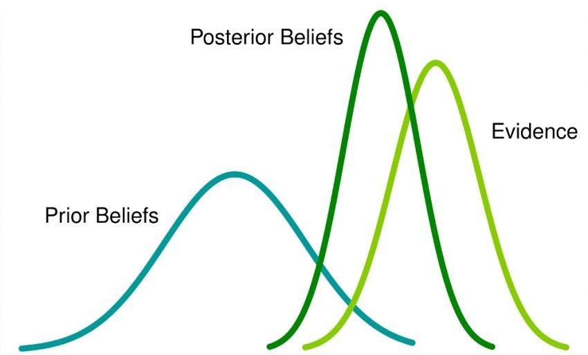
This approach involves initial “prior” beliefs (or probabilities) about an event which is updated when new evidence emerges through data collection. This results in ‘posterior’ beliefs which form the basis for Bayesian inferences. Often, people tend to overlook the prior probability of an event whereas posterior probability is always considered.
Before we actually delve deeper into Bayesian Statistics, let us briefly discuss Frequentist Statistics, the more popular version of statistics and the distinction between these two statistical philosophies.
In the realm of data science, Bayesian statistics serves as a powerful tool for inference and decision-making under uncertainty. Unlike traditional frequentist statistics, which relies on fixed parameters and p-values, Bayesian statistics provides a framework for updating beliefs based on new evidence. In this blog post, we will delve into the fundamental concepts of Bayesian statistics and explore its applications in data science, accompanied by illustrative graphs and code examples.
Understanding Bayesian Inference
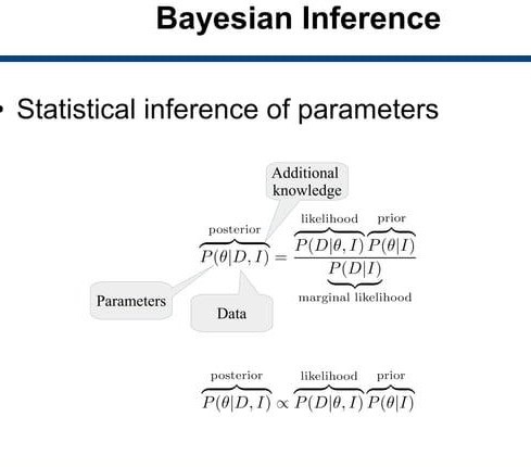
At the heart of Bayesian statistics lies the concept of Bayesian inference, which involves updating our beliefs about the parameters of interest in light of observed data. The key components of Bayesian inference include:
Prior Distribution: We start with an initial belief about the parameters, represented by a prior distribution. This distribution encapsulates our subjective knowledge or beliefs before observing any data.
Likelihood Function: The likelihood function quantifies the probability of observing the data given the parameters. It represents how well the parameters explain the observed data.
Posterior Distribution: Through Bayes’ theorem, the prior distribution is updated using the observed data to obtain the posterior distribution. The posterior distribution encapsulates our updated beliefs about the parameters after considering the observed data.
The Bayesian framework allows us to incorporate prior knowledge, if available, and update our beliefs as we gather more evidence.
Bayesian Inference in Action: Example
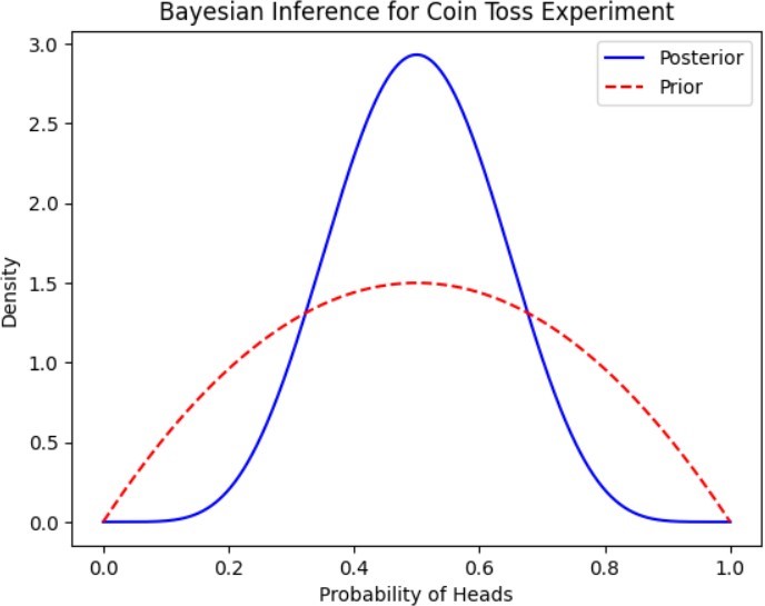
Let’s consider a simple example of Bayesian inference: estimating the probability of success in a coin toss experiment. We have a biased coin, and our goal is to infer the probability of obtaining heads (success).
Some basic concepts and applications of Bayesian statistics in data science are:
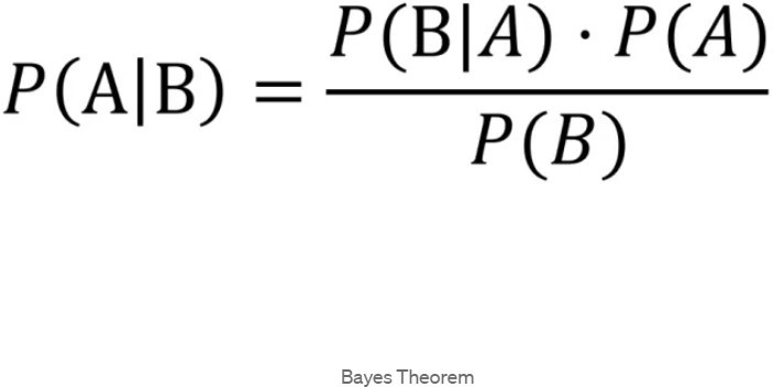
- Bayes’ rule: This is the fundamental equation of Bayesian inference, which allows us to update our beliefs about a hypothesis based on new It states that the posterior probability of a hypothesis given some data is proportional to the product of the prior probability of the hypothesis and the likelihood of the data given the hypothesis. Mathematically, it can be written as:
P(H∣D)∝P(H)P(D∣H)
where H is the hypothesis, D is the data, P(H) is the prior probability, P(D∣H) is the likelihood, and P(H∣D) is the posterior probability.
- Prior and posterior distributions: These are the probability distributions that represent our beliefs about a parameter or a variable before and after observing some data. The prior distribution reflects our initial assumptions or knowledge, while the posterior distribution incorporates the new information from the data. The posterior distribution can then be used as the prior distribution for further
- Likelihood function: This is the function that measures how well a hypothesis explains the observed It is proportional to the probability of the data given the hypothesis. The likelihood function can be used to compare different hypotheses and find the one that maximizes the fit to the data.
- Bayesian inference: This is the process of using Bayes’ rule to update our beliefs about a parameter or a variable based on new data. Bayesian inference can be done analytically, numerically, or using simulation methods such as Markov chain Monte Carlo (MCMC).
- Bayesian learning: This is the process of using Bayesian inference to learn from data and update our Bayesian learning can be used to estimate the parameters of a model, select the best model among a set of candidates, or discover the structure of a model from data.
- Bayesian prediction: This is the process of using Bayesian inference to make predictions about future or unseen data based on the current data and model. Bayesian prediction can be used to generate point estimates, interval estimates, or probability distributions for the predicted
Code Examples:
import numpy as np
import matplotlib.pyplot as plt from scipy.stats import beta
# Observed data (number of heads, number of tosses) data = np.array([5, 10])
# Define prior parameters (Beta distribution parameters) alpha_prior = 2
beta_prior = 2
# Compute posterior parameters alpha_posterior = alpha_prior + data[0] beta_posterior = beta_prior + data[1] – data[0]
# Generate posterior distribution
posterior = beta(alpha_posterior, beta_posterior)
# Plot prior and posterior distributions x = np.linspace(0, 1, 1000)
plt.plot(x, posterior.pdf(x), label=’Posterior’, color=’blue’)
plt.plot(x, beta(alpha_prior, beta_prior).pdf(x), label=’Prior’, color=’red’, linestyle=’–‘) plt.xlabel(‘Probability of Heads’)
plt.ylabel(‘Density’)
plt.title(‘Bayesian Inference for Coin Toss Experiment’) plt.legend()
plt.show()
Output:
Applications of Bayesian Statistics in Data Science
Bayesian statistics stands as a foundational pillar in modern data science, offering a principled framework for inference, modeling, and decision-making under uncertainty. Its versatility and robustness make it an invaluable tool across various domains. Below, we explore some of the key applications of Bayesian statistics in data science:
1. Parameter Estimation:
In data science, accurate parameter estimation forms the cornerstone of model building and inference. Bayesian statistics provides a rigorous approach to parameter estimation by
integrating prior knowledge with observed data to derive posterior distributions. This Bayesian paradigm is particularly beneficial in scenarios where data are scarce, noisy, or exhibit complex dependencies. Bayesian parameter estimation finds applications in fields ranging from Bayesian regression models in finance to Bayesian hierarchical models in epidemiology.
2. Hypothesis Testing:
Bayesian hypothesis testing offers a coherent alternative to classical frequentist methods by directly quantifying the probability of hypotheses given the data. By leveraging Bayes’ theorem, Bayesian hypothesis testing enables data scientists to evaluate competing hypotheses in a unified framework. Bayesian methods excel in scenarios where hypotheses are complex, uncertain, or require incorporating prior knowledge. Applications include A/B testing in online marketing, clinical trials in healthcare, and environmental impact assessments in ecology.
3. Machine Learning:
Bayesian techniques play a pivotal role in advancing the state-of-the-art in machine learning. Bayesian inference facilitates robust model training, uncertainty quantification, and model selection in complex learning tasks. Bayesian neural networks, Gaussian processes, and hierarchical Bayesian models are prominent examples of Bayesian techniques applied in machine learning. Bayesian approaches are particularly well-suited for applications such as anomaly detection, recommendation systems, and predictive maintenance in industrial settings.
4. Time Series Analysis:
Time series data, prevalent in domains like finance, meteorology, and signal processing, pose unique challenges due to temporal dependencies and inherent uncertainty. Bayesian time series models offer a flexible framework for capturing complex temporal patterns while accommodating uncertainty in predictions. Applications of Bayesian time series analysis include forecasting financial markets, predicting weather patterns, and monitoring sensor data in Internet of Things (IoT) devices.
5. Bayesian Networks:
Bayesian networks, also known as probabilistic graphical models, provide a powerful formalism for representing and reasoning about complex probabilistic relationships among variables.
Bayesian networks enable efficient inference and decision-making in domains characterized by uncertainty and interdependencies. Applications include fault diagnosis in engineering systems, risk assessment in healthcare, and fraud detection in financial transactions.
6. Bayesian Optimization:
Bayesian optimization is a sophisticated technique for global optimization of
expensive-to-evaluate objective functions. By constructing a probabilistic surrogate model of the objective function, Bayesian optimization intelligently selects the next evaluation point to balance exploration and exploitation. Applications range from hyperparameter tuning in machine learning algorithms to experimental design in scientific experiments and automated control in robotics.
Bayesian Statistics in Practice
1. Bayesian Linear Regression
import numpy as np
import matplotlib.pyplot as plt import pymc3 as pm
# Generate synthetic data np.random.seed(0)
X = np.linspace(0, 10, 100)
true_slope, true_intercept = 2, 1
Y = true_slope * X + true_intercept + np.random.normal(0, 1, size=len(X))
# Bayesian linear regression model with pm.Model() as linear_model:
# Priors for parameters
slope = pm.Normal(‘slope’, mu=0, sigma=10) intercept = pm.Normal(‘intercept’, mu=0, sigma=10) sigma = pm.HalfNormal(‘sigma’, sigma=1)
# Expected value of outcome mu = slope * X + intercept
# Likelihood
likelihood = pm.Normal(‘Y’, mu=mu, sigma=sigma, observed=Y)
# Sample posterior
trace = pm.sample(1000, tune=1000)
# Plot posterior distributions pm.traceplot(trace) plt.show()
Output:
2. Bayesian Model Selection
import numpy as np import pymc3 as pm
# Generate synthetic data np.random.seed(0)
X = np.linspace(0, 10, 100)
true_slope1, true_intercept1 = 2, 1
true_slope2, true_intercept2 = 3, 2
Y1 = true_slope1 * X + true_intercept1 + np.random.normal(0, 1, size=len(X)) Y2 = true_slope2 * X + true_intercept2 + np.random.normal(0, 1, size=len(X))
# Bayesian model selection
with pm.Model() as model_selection: # Priors for parameters
slope1 = pm.Normal(‘slope1’, mu=0, sigma=10) intercept1 = pm.Normal(‘intercept1’, mu=0, sigma=10) sigma1 = pm.HalfNormal(‘sigma1’, sigma=1)
slope2 = pm.Normal(‘slope2’, mu=0, sigma=10) intercept2 = pm.Normal(‘intercept2’, mu=0, sigma=10)
sigma2 = pm.HalfNormal(‘sigma2’, sigma=1)
# Expected values of outcomes mu1 = slope1 * X + intercept1 mu2 = slope2 * X + intercept2
# Likelihood for model 1
likelihood1 = pm.Normal(‘Y1’, mu=mu1, sigma=sigma1, observed=Y1)
# Likelihood for model 2
likelihood2 = pm.Normal(‘Y2’, mu=mu2, sigma=sigma2, observed=Y2)
# Compute marginal likelihoods
marginal_likelihood1 = pm.sample_posterior_predictive(trace, samples=1000, model=linear_model)
marginal_likelihood2 = pm.sample_posterior_predictive(trace, samples=1000, model=model_selection)
3. Bayesian Neural Networks
import numpy as np import tensorflow as tf
import tensorflow_probability as tfp
import matplotlib.pyplot as plt tfd = tfp.distributions
# Generate synthetic data np.random.seed(0)
X = np.linspace(0, 10, 100)
true_slope, true_intercept = 2, 1
Y = true_slope * X + true_intercept + np.random.normal(0, 1, size=len(X))
# Define Bayesian Neural Network model model = tf.keras.Sequential([
tf.keras.layers.Dense(10, activation=’relu’), tfp.layers.DenseFlipout(1)
])
# Define negative log likelihood loss function def negative_log_likelihood(y_true, y_pred):
return -y_pred.distribution.log_prob(y_true)
# Compile the model
model.compile(optimizer=tf.optimizers.Adam(learning_rate=0.01), loss=negative_log_likelihood)
# Convert data to tensors
X_tensor = tf.convert_to_tensor(X.reshape(-1, 1), dtype=tf.float32) Y_tensor = tf.convert_to_tensor(Y.reshape(-1, 1), dtype=tf.float32)
# Train the model
history = model.fit(X_tensor, Y_tensor, epochs=1000, verbose=0)
# Plot training history plt.plot(history.history[‘loss’]) plt.xlabel(‘Epochs’)
plt.ylabel(‘Negative Log Likelihood Loss’) plt.title(‘Training History’)
plt.show()
Conclusion
In conclusion, delving into Bayesian statistics unveils a rich landscape of inference, decision-making, and uncertainty quantification in the realm of data science. Through this
exploration, we have traversed fundamental concepts, including prior distributions, likelihood functions, and posterior distributions, which form the backbone of Bayesian inference.
Bayesian statistics stands as a beacon of principled reasoning, offering a holistic framework for incorporating prior knowledge and updating beliefs based on observed data. Unlike frequentist approaches, which often rely solely on point estimates and hypothesis testing, Bayesian methodology provides a nuanced understanding of uncertainty, essential for robust
decision-making in complex real-world scenarios.
The practical applications of Bayesian statistics in data science are manifold. From parameter estimation and hypothesis testing to machine learning and time series analysis, Bayesian methods empower data scientists to extract meaningful insights from data while acknowledging and quantifying inherent uncertainty.
The inclusion of code examples and graphical representations in this discussion underscores the accessibility and applicability of Bayesian techniques in practice. By leveraging Python libraries such as NumPy, SciPy, and Matplotlib, practitioners can seamlessly implement Bayesian models, visualize results, and gain deeper insights into their data.
As we navigate the ever-evolving landscape of data science, Bayesian statistics remains a steadfast ally, guiding us through the intricacies of uncertainty and facilitating informed decision-making. Embracing Bayesian principles empowers us to navigate ambiguity with confidence, uncover hidden patterns within data, and drive actionable insights that propel organizations forward.
In essence, Bayesian statistics transcends mere methodology; it embodies a paradigm shift—a commitment to probabilistic reasoning, continual learning, and evidence-based decision-making. As data scientists, let us embrace the Bayesian ethos, harnessing its power to unravel the mysteries of data and illuminate pathways to knowledge and discovery.
In the journey ahead, may Bayesian statistics serve as both a compass and a companion, guiding us toward deeper understanding, richer insights, and transformative impact in the dynamic landscape of data science.