Introduction to Supervised Machine Learning

Supervised learning is a machine learning technique that is widely used in various fields such as finance, healthcare, marketing, and more. It is a form of machine learning in which the algorithm is trained on labelled data to make predictions or decisions based on the data inputs. In supervised learning, the algorithm learns a mapping between the input and output data. This mapping is learned from a labelled dataset, which consists of pairs of input and output data. The algorithm tries to learn the relationship between the input and output data so that it can make accurate predictions on new, unseen data.

Linear Regression in Machine Learning:

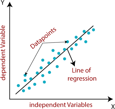
Linear regression algorithm shows a linear relationship between a dependent (y) and one or more independent (y) variables, hence called as linear regression. Since linear regression shows the linear relationship, which means it finds how the value of the dependent variable is changing according to the value of the independent variable. Linear regression makes predictions for continuous/real or numeric variables such as sales, salary, age, product price, etc. The linear regression model provides a sloped straight line representing the relationship between the variables. Consider the below image:

Mathematically, we can represent a linear regression as:

To calculate best-fit line linear regression uses a traditional slope-intercept form. y= Dependent Variable.

y= Dependent Variable

x= Independent Variable.

a0= intercept of the line.

a1 = Linear regression coefficient(slope).

Need of a Linear regression:

As mentioned above, Linear regression estimates the relationship between a dependent variable and an independent variable. Let’s understand this with an easy example:

Let’s say we want to estimate the salary of an employee based on year of experience. You have the recent company data, which indicates the relationship between experience and salary. Here year of experience is an independent variable, and the salary of an employee is a dependent variable, as the salary of an employee is dependent on the experience of an employee. Using this insight, we can predict the future salary of the employee based on current & past information.

Gradient Descent:

A linear regression model can be trained using the optimization algorithm gradient descent by iteratively modifying the model’s parameters to reduce the mean squared error (MSE) of the model on a training dataset. To update a0 and a1 values in order to reduce the Cost function (minimizing RMSE value) and achieve the best-fit line the model uses Gradient Descent. The idea is to start with random θ₁ and θ₂ values and then iteratively update the values, reaching minimum cost.

A gradient is nothing but a derivative that defines the effects on outputs of the function with a little bit of variation in inputs.

Finding the coefficients of a linear equation that best fits the training data is the objective of linear regression. By moving in the direction of the Mean Squared Error negative gradient with respect to the coefficients, the coefficients can be changed. And the respective intercept and coefficient of X will be if is the learning rate. In Linear Regression, Mean Squared Error (MSE) cost function is used, which is the average of squared error that occurred between the predicted values and actual values.

Logistic Regression in Machine Learning:

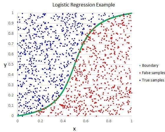
Logistic regression is a supervised machine learning algorithm mainly used for classification tasks where the goal is to predict the probability that an instance of belonging to a given class. It is used for classification algorithms its name is logistic regression. it’s referred to as regression because it takes the output of the linear regression function as input and uses a sigmoid function to estimate the probability for the given class. The difference between linear regression and logistic regression is that linear regression output is the continuous value that can be anything while logistic regression predicts the probability that an instance belongs to a given class or not.

Logistic Regression:

• Using logistic regression, the result of a categorical dependent variable is As a result, a discrete or category value must be the result.
• Instead of providing the exact values, which are 0 and 1, it provides the probabilistic values, which fall between 0 and 1. It can be either Yes or No, 0 or 1, true or False,
• Instead of constructing a regression line, we fit a “S” shaped logistic function, which predicts one of two maximum values (0 or 1).
• The logistic function curve reflects the possibility of something such as whether the cells are cancerous or not, whether a mouse is obese or not based on its weight, and so on.
• Logistic Regression is an important machine learning approach because it can generate probabilities and classify new data using both continuous and discrete
• Logistic Regression can be used to categorize observations using many forms of data and can quickly find which factors are most efficient for

Logistic Regression Equation:

The mathematical steps to get Logistic Regression equations are given below: We know the equation of the straight line can be written as:

In Logistic Regression y can be between 0 and 1 only, so for this let’s divide the above equation by (1-y):

But we need range between -[infinity] to +[infinity], then take logarithm of the equation it will become:

Type of Logistic Regression:

On the basis of the categories, Logistic Regression can be classified into three types:

• Binomial: In binomial Logistic regression, there can be only two possible types of the dependent variables, such as 0 or 1, Pass or Fail,
• Multinomial: In multinomial Logistic regression, there can be 3 or more possible unordered types of the dependent variable, such as “cat”, “dogs”, or “sheep”
• Ordinal: In ordinal Logistic regression, there can be 3 or more possible ordered types of dependent variables, such as “low”, “Medium”, or “High”.

Here are some common terms involved in logistic regression:

• Independent variables: The input features or predictor factors used to make predictions for the dependent
• Dependent variable: The dependent variable in a logistic regression model is the variable that we are attempting to
• Logistic function: The formula used to depict how the independent and dependent variables relate to one another. The logistic function converts the input variables into a probability value between 0 and 1, which represents the possibility of the dependent variable being 1 or
• Odds: Odds are the ratio of something happening to something not happening. It differs from probability in that probability is the ratio of anything happening to everything that could
• Coefficient: The estimated parameters of the logistic regression model illustrate how the independent and dependent variables relate to one
• Intercept: In the logistic regression model, a constant factor that represents the log chances when all independent variables are equal to

Decision Tree Algorithm:

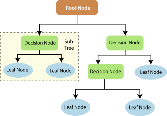
A decision tree is a strong tool in supervised learning algorithms that may be utilized for both classification and regression applications. It creates a flowchart-like tree structure, with each internal node representing a test on an attribute, each branch representing a test outcome, and each leaf node (terminal node) holding a class label. It is built by iteratively splitting the training data into subsets depending on attribute values until a stopping requirement, such as the maximum depth of the tree or the minimum number of samples needed to divide a node, is met.

The Decision Tree method determines the appropriate attribute to split the data during training based on a metric such as entropy or Gini impurity, which quantifies the level of impurity or unpredictability in the subsets. The goal is to determine the property that optimizes information gain or impurity reduction following the split.

Decision Tree Terminologies:

Some of the common Terminologies used in Decision Trees are as follows:

• Root Node: The root node is the topmost node in the tree and represents the entire It is the beginning point for decision-making.
• Decision/Internal Node: Decision/Internal Node: A node that represents a decision on an input Internal nodes that branch off connect to leaf nodes or other internal nodes.
• Leaf/Terminal Node: Leaf/Terminal Node: A node that has no child nodes and represents a class label or a number
• Splitting: The process of dividing a node into two or more sub-nodes based on a split criterion and a chosen
• Branch/Sub-Tree: A subsection of the decision tree begins at an internal node and finishes at the leaf
• Parent Node: The node that divides into one or more child nodes is known as the parent
• Child Node: The nodes that develop when a parent node is divided are referred to as child
• Impurity: A measure of the homogeneity of the target variable in a subset of data. It denotes the degree of unpredictability or uncertainty in a collection of The Gini index and entropy are two impurity metrics often used in decision trees for classification tasks.
• Variance: Variance measures how much the anticipated and target variables change across samples of a dataset. It is used in decision trees for regression situations. The variance for the regression tasks in the decision tree is measured using mean squared error, mean absolute error, friedman_mse, or half Poisson
• Information Gain: Information gain is a measure of the impurity reduction obtained by dividing a dataset on a certain feature in a decision tree. The feature that provides the largest information gain is used to find the most informative feature to split on at each node of the tree, with the goal of constructing pure
• Pruning: The process of removing branches from a tree that provide no extra information or result in

How does the Decision Tree algorithm Work?

The decision tree operates by analysing the data set to predict its classification. It commences from the tree’s root node, where the algorithm views the value of the root attribute compared to the attribute of the record in the actual data set. Based on the comparison, it proceeds to follow the branch and move to the next node.

The algorithm repeats this action for every subsequent node by comparing its attribute values with those of the sub-nodes and continuing the process further. It repeats until it reaches the leaf node of the tree. The complete mechanism can be better explained through the algorithm given below.

• Step-1: Begin the tree with the root node, says S, which contains the complete
• Step-2: Find the best attribute in the dataset using Attribute Selection Measure (ASM).
• Step-3: Divide the S into subsets that contains possible values for the best
• Step-4: Generate the decision tree node, which contains the best
• Step-5: Recursively make new decision trees using the subsets of the dataset created in step -3. Continue this process until a stage is reached where you cannot further classify the nodes and called the final node as a leaf node Classification and Regression Tree

Advantages of the Decision Tree:

1. It is simple to understand as it follows the same process which a human follow while making any decision in real-life.
2. It can be very useful for solving decision-related
3. It helps to think about all the possible outcomes for a
4. There is less requirement of data cleaning compared to other

Disadvantages of the Decision Tree:

1. The decision tree contains lots of layers, which makes it
2. It may have an overfitting issue, which can be resolved using the Random Forest
3. For more class labels, the computational complexity of the decision tree may

Random Forest Algorithm:

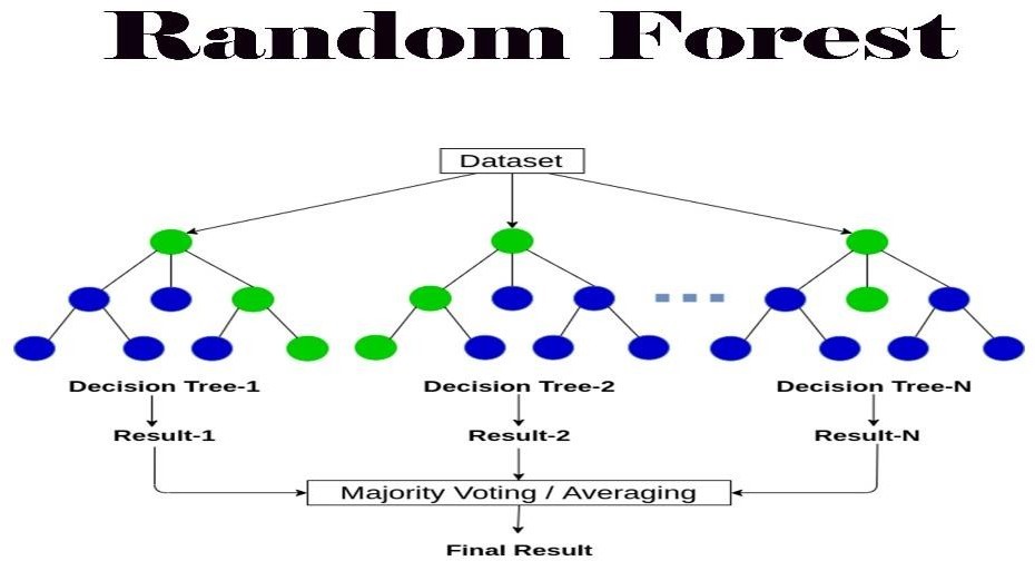
Random Forest is an ensemble technique that can handle both regression and classification tasks by combining many decision trees and a technique known as Bootstrap and Aggregation, or bagging. The core idea is to use numerous decision trees to determine the final output rather than depending on individual decision trees.

Random Forest’s foundation learning models are numerous decision trees. We randomly select rows and features from the dataset to create sample datasets for each model. This section is known as Bootstrap.

We must approach the Random Forest regression strategy in the same way as we would any other machine learning technique.

Why use Random Forest?

Below are some points that explain why we should use the Random Forest algorithm:

• It takes less training time as compared to other
• It predicts output with high accuracy, even for the large dataset it runs
• It can also maintain accuracy when a large proportion of data is missing

How does Random Forest algorithm work?

Random Forest works in two-phase first is to create the random forest by combining N decision tree, and second is to make predictions for each tree created in the first phase.

The Working process can be explained in the below steps and diagram:

Step-1: Select random K data points from the training set.

Step-2: Build the decision trees associated with the selected data points (Subsets).

Step-3: Choose the number N for decision trees that you want to build.

Step-4: Repeat Step 1 & 2.

Step-5: For new data points, find the predictions of each decision tree, and assign the new data points to the category that wins the majority votes.

Applications of Random Forest:

There are mainly four sectors where Random Forest mostly used:

1. Banking: Banking sector mostly uses this algorithm for the identification of loan risk.
2. Medicine: With the help of this algorithm, disease trends and risks of the disease can be
3. Land Use: We can identify the areas of similar land use by this
4. Marketing: Marketing trends can be identified using this algorithm.

Advantages of Random Forest:

• Random Forest is capable of performing both Classification and Regression
• It is capable of handling large datasets with high
• It enhances the accuracy of the model and prevents the overfitting

Disadvantages of Random Forest:

• The model can also be difficult to
• This algorithm may require some domain expertise to choose the appropriate parameters like the number of decision trees, the maximum depth of each tree, and the number of features to consider at each
• It is computationally expensive, especially for large
• It may suffer from overfitting if the model is too complex or the number of decision trees is too